E-commerce Data Analysis Part One - Data Wrangling & Monthly Revenue
10 Nov 2020Introduction:
In this E-commerce Data Series, we will analyze sales data from a UK online retialer. In part one, we will be mainly focus on the data wrangling and then move on to caculate the monthly revenue growth rate.
Table Of Content:
- Exploratory Data Analysis
- Data Cleaning
- Monthly Revenue Growth
Prepare to Take-Off
# Setting up the environment
import pandas as pd
import numpy as np
import datetime as dt
import matplotlib.pyplot as plt
from operator import attrgetter
import seaborn as sns
import matplotlib.colors as mcolors
Exploratory Data Analysis
# Import Data
data = pd.read_csv("OnlineRetail.csv",engine="python")
data.info()
<class 'pandas.core.frame.DataFrame'>
RangeIndex: 541909 entries, 0 to 541908
Data columns (total 8 columns):
InvoiceNo      541909 non-null object
StockCode      541909 non-null object
Description    540455 non-null object
Quantity       541909 non-null int64
InvoiceDate    541909 non-null object
UnitPrice      541909 non-null float64
CustomerID     406829 non-null float64
Country        541909 non-null object
dtypes: float64(2), int64(1), object(5)
memory usage: 33.1+ MB
It’s better to change $InvoiceDate$ column in to $datatime64(ns)$ types for future data analysis on monthly revenue growth. In this project, we would ignore the hours and minutes within $InvoiceDate$ column, only the day,month,year will be stored in the dataframe.
# Change InvoiceDate data type
data['InvoiceDate'] = pd.to_datetime(data['InvoiceDate'])
# Convert to InvoiceDate hours to the same mid-night time.
data['date']=data['InvoiceDate'].dt.normalize()
# Check Data Type
data.info()
<class 'pandas.core.frame.DataFrame'>
RangeIndex: 541909 entries, 0 to 541908
Data columns (total 9 columns):
InvoiceNo      541909 non-null object
StockCode      541909 non-null object
Description    540455 non-null object
Quantity       541909 non-null int64
InvoiceDate    541909 non-null datetime64[ns]
UnitPrice      541909 non-null float64
CustomerID     406829 non-null float64
Country        541909 non-null object
date           541909 non-null datetime64[ns]
dtypes: datetime64[ns](2), float64(2), int64(1), object(4)
memory usage: 37.2+ MB
# Summerize the null value in dataframe.
print(data.isnull().sum())
# Missing values percentage
missing_percentage = data.isnull().sum() / data.shape[0] * 100
missing_percentage
InvoiceNo           0
StockCode           0
Description      1454
Quantity            0
InvoiceDate         0
UnitPrice           0
CustomerID     135080
Country             0
date                0
dtype: int64


InvoiceNo       0.000000
StockCode       0.000000
Description     0.268311
Quantity        0.000000
InvoiceDate     0.000000
UnitPrice       0.000000
CustomerID     24.926694
Country         0.000000
date            0.000000
dtype: float64
Around 25% of rows wihtin $CustomerID$ column is missing values, this would impose a question mark on the implementation of digital tracking system for any business. We normally would look into more details but in this case, we do not have any visibilities on them. Let’s continue to explore the missing values in $Description$ and $UnitPrice$ Column.
data[data.Description.isnull()].head()
| InvoiceNo | StockCode | Description | Quantity | InvoiceDate | UnitPrice | CustomerID | Country | date | |
|---|---|---|---|---|---|---|---|---|---|
| 622 | 536414 | 22139 | NaN | 56 | 2010-12-01 11:52:00 | 0.0 | NaN | United Kingdom | 2010-12-01 |
| 1970 | 536545 | 21134 | NaN | 1 | 2010-12-01 14:32:00 | 0.0 | NaN | United Kingdom | 2010-12-01 |
| 1971 | 536546 | 22145 | NaN | 1 | 2010-12-01 14:33:00 | 0.0 | NaN | United Kingdom | 2010-12-01 |
| 1972 | 536547 | 37509 | NaN | 1 | 2010-12-01 14:33:00 | 0.0 | NaN | United Kingdom | 2010-12-01 |
| 1987 | 536549 | 85226A | NaN | 1 | 2010-12-01 14:34:00 | 0.0 | NaN | United Kingdom | 2010-12-01 |
# How often a record without description is also missing unit price information and customerID
data[data.Description.isnull()].CustomerID.isnull().value_counts()
True    1454
Name: CustomerID, dtype: int64
data[data.Description.isnull()].UnitPrice.isnull().value_counts()
False    1454
Name: UnitPrice, dtype: int64
data[data.CustomerID.isnull()].head()
| InvoiceNo | StockCode | Description | Quantity | InvoiceDate | UnitPrice | CustomerID | Country | date | |
|---|---|---|---|---|---|---|---|---|---|
| 622 | 536414 | 22139 | NaN | 56 | 2010-12-01 11:52:00 | 0.00 | NaN | United Kingdom | 2010-12-01 |
| 1443 | 536544 | 21773 | DECORATIVE ROSE BATHROOM BOTTLE | 1 | 2010-12-01 14:32:00 | 2.51 | NaN | United Kingdom | 2010-12-01 |
| 1444 | 536544 | 21774 | DECORATIVE CATS BATHROOM BOTTLE | 2 | 2010-12-01 14:32:00 | 2.51 | NaN | United Kingdom | 2010-12-01 |
| 1445 | 536544 | 21786 | POLKADOT RAIN HAT | 4 | 2010-12-01 14:32:00 | 0.85 | NaN | United Kingdom | 2010-12-01 |
| 1446 | 536544 | 21787 | RAIN PONCHO RETROSPOT | 2 | 2010-12-01 14:32:00 | 1.66 | NaN | United Kingdom | 2010-12-01 |
data.loc[data.CustomerID.isnull(), ["UnitPrice", "Quantity"]].describe()
| UnitPrice | Quantity | |
|---|---|---|
| count | 135080.000000 | 135080.000000 |
| mean | 8.076577 | 1.995573 |
| std | 151.900816 | 66.696153 |
| min | -11062.060000 | -9600.000000 |
| 25% | 1.630000 | 1.000000 |
| 50% | 3.290000 | 1.000000 |
| 75% | 5.450000 | 3.000000 |
| max | 17836.460000 | 5568.000000 |
It is fair to say ‘UnitePirce’ and ‘Quantity’ column shows extreme outliers. As we need to use historical purhcase price and quantity to make sale forcast in the future, these outliers can be disruptive. Therefore, let us dorp of the null values. Besides dropping all the missing values in description column. How about the hidden values? like ‘nan’ instead of ‘NaN’. In the next following steps we will drop any rows with ‘nan’ and ‘’ strings in it.
Data Cleaning - Dropping Rows With Missing Values
# Can we find any hidden Null values? "nan"-Strings? in Description
data.loc[data.Description.isnull()==False, "lowercase_descriptions"] =  data.loc[
    data.Description.isnull()==False,"Description"].apply(lambda l: l.lower())

data.lowercase_descriptions.dropna().apply(
    lambda l: np.where("nan" in l, True, False)).value_counts()
False    539724
True        731
Name: lowercase_descriptions, dtype: int64
# How about "" in Description?
data.lowercase_descriptions.dropna().apply(
    lambda l: np.where("" == l, True, False)).value_counts()
False    540455
Name: lowercase_descriptions, dtype: int64
# Transform "nan" toward "NaN"
data.loc[data.lowercase_descriptions.isnull()==False, "lowercase_descriptions"] = data.loc[
    data.lowercase_descriptions.isnull()==False, "lowercase_descriptions"
].apply(lambda l: np.where("nan" in l, None, l))
# Verified all the 'nan' changed into 'Nan'
data.lowercase_descriptions.dropna().apply(lambda l: np.where("nan" in l, True, False)).value_counts()
False    539724
Name: lowercase_descriptions, dtype: int64
#drop all the null values and hidden-null values
data.loc[(data.CustomerID.isnull()==False)&(data.lowercase_descriptions.isnull()==False)].info()
<class 'pandas.core.frame.DataFrame'>
Int64Index: 406223 entries, 0 to 541908
Data columns (total 10 columns):
InvoiceNo                 406223 non-null object
StockCode                 406223 non-null object
Description               406223 non-null object
Quantity                  406223 non-null int64
InvoiceDate               406223 non-null datetime64[ns]
UnitPrice                 406223 non-null float64
CustomerID                406223 non-null float64
Country                   406223 non-null object
date                      406223 non-null datetime64[ns]
lowercase_descriptions    406223 non-null object
dtypes: datetime64[ns](2), float64(2), int64(1), object(5)
memory usage: 34.1+ MB
# data without any null values
data_clean = data.loc[(data.CustomerID.isnull()==False)&(data.lowercase_descriptions.isnull()==False)].copy()
data_clean.isnull().sum().sum()
0
Monthly Revenue Growth
# Create Revenue Column
data_clean['Revenue'] = data_clean['UnitPrice'] * data_clean['Quantity']
# Create YearMonth Column
data_clean['YearMonth'] = data_clean['InvoiceDate'].apply(lambda date: date.year*100+date.month)
data_clean.head(n=5)
| InvoiceNo | StockCode | Description | Quantity | InvoiceDate | UnitPrice | CustomerID | Country | date | lowercase_descriptions | Revenue | YearMonth | |
|---|---|---|---|---|---|---|---|---|---|---|---|---|
| 0 | 536365 | 85123A | WHITE HANGING HEART T-LIGHT HOLDER | 6 | 2010-12-01 08:26:00 | 2.55 | 17850.0 | United Kingdom | 2010-12-01 | white hanging heart t-light holder | 15.30 | 201012 |
| 1 | 536365 | 71053 | WHITE METAL LANTERN | 6 | 2010-12-01 08:26:00 | 3.39 | 17850.0 | United Kingdom | 2010-12-01 | white metal lantern | 20.34 | 201012 |
| 2 | 536365 | 84406B | CREAM CUPID HEARTS COAT HANGER | 8 | 2010-12-01 08:26:00 | 2.75 | 17850.0 | United Kingdom | 2010-12-01 | cream cupid hearts coat hanger | 22.00 | 201012 |
| 3 | 536365 | 84029G | KNITTED UNION FLAG HOT WATER BOTTLE | 6 | 2010-12-01 08:26:00 | 3.39 | 17850.0 | United Kingdom | 2010-12-01 | knitted union flag hot water bottle | 20.34 | 201012 |
| 4 | 536365 | 84029E | RED WOOLLY HOTTIE WHITE HEART. | 6 | 2010-12-01 08:26:00 | 3.39 | 17850.0 | United Kingdom | 2010-12-01 | red woolly hottie white heart. | 20.34 | 201012 |
#monthly data using pivot table.
df_monthly = data_clean.copy()
df_monthly = pd.pivot_table(data_clean,index=['YearMonth'],values="Revenue",aggfunc=[np.sum])
print(df_monthly)
                   sum
               Revenue
YearMonth
201012      554314.170
201101      474834.980
201102      435859.050
201103      578790.310
201104      425132.101
201105      647536.030
201106      607671.010
201107      573614.931
201108      615532.500
201109      930559.562
201110      973348.740
201111     1130196.310
201112      342039.000
# Groupby 'YearMonth' Column
df_monthly_more = data_clean.groupby('YearMonth').agg({'CustomerID':lambda x: x.nunique(), 'Quantity': 'sum',\
                                                       'Revenue': 'sum',}).reset_index()
print(df_monthly_more)
    YearMonth  CustomerID  Quantity      Revenue
0      201012       948.0    296153   554314.170
1      201101       783.0    269219   474834.980
2      201102       798.0    262381   435859.050
3      201103      1020.0    343284   578790.310
4      201104       899.0    278050   425132.101
5      201105      1079.0    367411   647536.030
6      201106      1051.0    356715   607671.010
7      201107       993.0    363027   573614.931
8      201108       980.0    386080   615532.500
9      201109      1302.0    536963   930559.562
10     201110      1425.0    568919   973348.740
11     201111      1711.0    668568  1130196.310
12     201112       685.0    203554   342039.000
# Create MonthlyGrowth Column:
df_monthly_more['MonthlyGrowth'] = df_monthly_more['Revenue'].pct_change()
import seaborn as sns
sns.set_style("whitegrid")
sns.catplot(x="YearMonth", y="Revenue", data=df_monthly_more, kind="point", aspect=2.5, color="#95a5a6")
plt.ylabel('Revenue')
plt.xlabel('')
sns.despine(left=True, bottom=True)

df_monthly_more.style.format({"Customers": "{:.0f}", \
                         "Quantity": "{:.0f}",\
                         "Revenue": "${:.0f}",\
                        "MonthlyGrowth": "{:.2f}"})\
                    .bar(subset=["Revenue",], color='lightgreen')\
                    .bar(subset=["CustomerID"], color='#FFA07A')
| YearMonth | CustomerID | Quantity | Revenue | MonthlyGrowth | |
|---|---|---|---|---|---|
| 0 | 201012 | 948 | 296153 | $554314 | nan |
| 1 | 201101 | 783 | 269219 | $474835 | -0.14 |
| 2 | 201102 | 798 | 262381 | $435859 | -0.08 |
| 3 | 201103 | 1020 | 343284 | $578790 | 0.33 |
| 4 | 201104 | 899 | 278050 | $425132 | -0.27 |
| 5 | 201105 | 1079 | 367411 | $647536 | 0.52 |
| 6 | 201106 | 1051 | 356715 | $607671 | -0.06 |
| 7 | 201107 | 993 | 363027 | $573615 | -0.06 |
| 8 | 201108 | 980 | 386080 | $615533 | 0.07 |
| 9 | 201109 | 1302 | 536963 | $930560 | 0.51 |
| 10 | 201110 | 1425 | 568919 | $973349 | 0.05 |
| 11 | 201111 | 1711 | 668568 | $1130196 | 0.16 |
| 12 | 201112 | 685 | 203554 | $342039 | -0.70 |
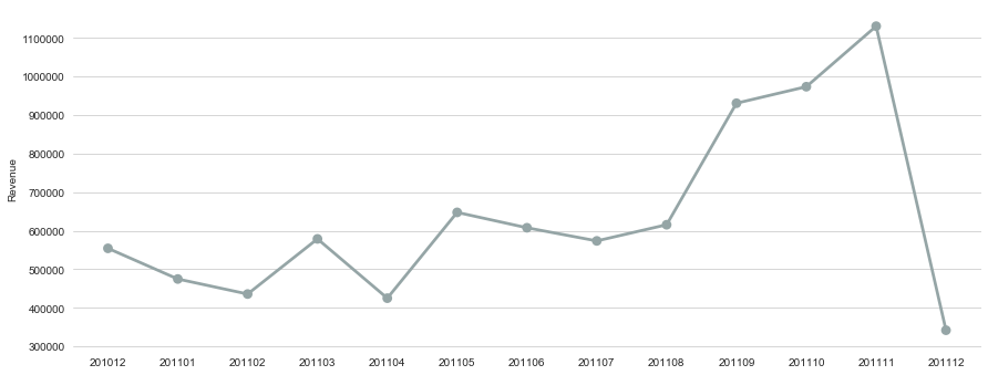
Conclusion:
The monthly revenue fluctuates over time and we see a sharp decline in Dec 2011. Since we do not have full month data in December 2011, the monthly revenue in Dec is much lower than previous months. From the line graph, we also saw a drop in the spring of 2011. These fluctuation may caused by credit card debts which were accumulated in previous Christmas season. Customers might also needs to file their tax during spring. In general, the E-commerce revenue is booming for this retailer, revenue from 2010 to 2011 is going upwards and we saw a major breakthourgh for 51% month to month growth in Sep.
The next question we need to ask: How many customer decide to come back and purchase from this retailer?
In the next post, we will look into the customer cohort and retention rate.