E-commerce Data Analysis Part Two - Customer Cohort Analysis
12 Nov 2020Introduction:
In E-commerce Data Series Part Two, we will mainly focus on customer cohort analysis. In part one, we already went through data cleaning process, so we would follow the same steps here. There are many benefits to adopt cohort analysis. In my personal opinion, the main goal we are trying to achieve in Cohort Analysis is form a better understanding of how customer behavior have affect on business.
In this Ecommerce case, we would like to know:
- How much revenue new customers bring to the business compared to the existing customers?
- What’s the customer retention rate for different cohort group?
Why these two question is so important to this business? Because it’s more expensive to acquire a new customer than keeping a warm customer who pruchased items on the business. We would love to see our customer base expanding over time and re-curring revenue increasing.
Table Of Content:
- Data Wrangling
- New vs. Existing Customer
- Cohort Analysis
Data Wrangling - Exploratory Data Analysis
# Setting up the environment
import pandas as pd
import numpy as np
import datetime as dt
import matplotlib.pyplot as plt
from operator import attrgetter
import seaborn as sns
import matplotlib.colors as mcolors

# Import Data
data = pd.read_csv("OnlineRetail.csv",engine="python")
data.info()

# Change InvoiceDate data type
data['InvoiceDate'] = pd.to_datetime(data['InvoiceDate'])
# Convert to InvoiceDate hours to the same mid-night time.
data['date']=data['InvoiceDate'].dt.normalize()

# Summerize the null value in dataframe.
print(data.isnull().sum())
# Missing values percentage
missing_percentage = data.isnull().sum() / data.shape[0] * 100
<class 'pandas.core.frame.DataFrame'>
RangeIndex: 541909 entries, 0 to 541908
Data columns (total 8 columns):
InvoiceNo      541909 non-null object
StockCode      541909 non-null object
Description    540455 non-null object
Quantity       541909 non-null int64
InvoiceDate    541909 non-null object
UnitPrice      541909 non-null float64
CustomerID     406829 non-null float64
Country        541909 non-null object
dtypes: float64(2), int64(1), object(5)
memory usage: 33.1+ MB
InvoiceNo           0
StockCode           0
Description      1454
Quantity            0
InvoiceDate         0
UnitPrice           0
CustomerID     135080
Country             0
date                0
dtype: int64
data.loc[data.CustomerID.isnull(), ["UnitPrice", "Quantity"]].describe()
| UnitPrice | Quantity | |
|---|---|---|
| count | 135080.000000 | 135080.000000 |
| mean | 8.076577 | 1.995573 |
| std | 151.900816 | 66.696153 |
| min | -11062.060000 | -9600.000000 |
| 25% | 1.630000 | 1.000000 |
| 50% | 3.290000 | 1.000000 |
| 75% | 5.450000 | 3.000000 |
| max | 17836.460000 | 5568.000000 |
It is fair to say ‘UnitePirce’ and ‘Quantity’ column shows extreme outliers. As we need to use historical purhcase price and quantity to make sale forcast in the future, these outliers can be disruptive. Therefore, let us dorp of the null values. Besides dropping all the missing values in description column. How about the hidden values? like ‘nan’ instead of ‘NaN’. In the next following steps we will drop any rows with ‘nan’ and ‘’ strings in it.
Data Cleaning - Dropping Rows With Missing Values
# Can we find any hidden Null values? "nan"-Strings? in Description
data.loc[data.Description.isnull()==False, "lowercase_descriptions"] =  data.loc[
    data.Description.isnull()==False,"Description"].apply(lambda l: l.lower())

data.lowercase_descriptions.dropna().apply(
    lambda l: np.where("nan" in l, True, False)).value_counts()
False    539724
True        731
Name: lowercase_descriptions, dtype: int64
# How about "" in Description?
data.lowercase_descriptions.dropna().apply(
    lambda l: np.where("" == l, True, False)).value_counts()
False    540455
Name: lowercase_descriptions, dtype: int64
# Transform "nan" toward "NaN"
data.loc[data.lowercase_descriptions.isnull()==False, "lowercase_descriptions"] = data.loc[
    data.lowercase_descriptions.isnull()==False, "lowercase_descriptions"
].apply(lambda l: np.where("nan" in l, None, l))

# Verified all the 'nan' changed into 'Nan'
data.lowercase_descriptions.dropna().apply(lambda l: np.where("nan" in l, True, False)).value_counts()
False    539724
Name: lowercase_descriptions, dtype: int64
#drop all the null values and hidden-null values
data.loc[(data.CustomerID.isnull()==False)&(data.lowercase_descriptions.isnull()==False)].info()

# data without any null values
data_clean = data.loc[(data.CustomerID.isnull()==False)&(data.lowercase_descriptions.isnull()==False)].copy()
data_clean.isnull().sum().sum()
<class 'pandas.core.frame.DataFrame'>
Int64Index: 406223 entries, 0 to 541908
Data columns (total 10 columns):
InvoiceNo                 406223 non-null object
StockCode                 406223 non-null object
Description               406223 non-null object
Quantity                  406223 non-null int64
InvoiceDate               406223 non-null datetime64[ns]
UnitPrice                 406223 non-null float64
CustomerID                406223 non-null float64
Country                   406223 non-null object
date                      406223 non-null datetime64[ns]
lowercase_descriptions    406223 non-null object
dtypes: datetime64[ns](2), float64(2), int64(1), object(5)
memory usage: 34.1+ MB


0
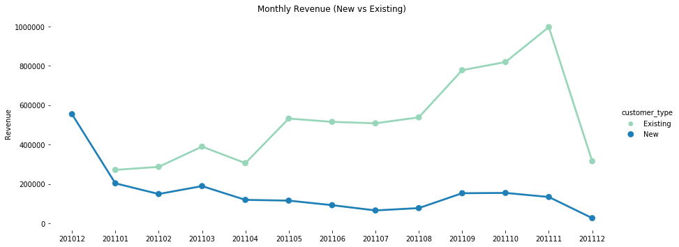
New Customer Vs Existing
In this Project, we defined the Existing customers as the group of records with lastest $FirstConversion$ later than the $FirstConversionYearMonth$. In other words, a existing customer should have purchase history with InvoiceDate later than their first purchase date. Since we only have part of the Dec data, a lower than average monthly revenue number from Dec 2011 was expected.
# Create Revenue Column
data_clean['Revenue'] = data_clean['UnitPrice'] * data_clean['Quantity']

# Create YearMonth Column
data_clean['YearMonth'] = data_clean['InvoiceDate'].apply(lambda date: date.year*100+date.month)

# New Vs. Existing
first_conversion = data_clean.groupby('CustomerID').agg({'InvoiceDate': lambda x: x.min()}).reset_index()
first_conversion.columns = ['CustomerID','FirstConversion']

# Change the Strings in FirstConversion Column into 'YearMonth' format number.
first_conversion['FirstConversionYearMonth'] = first_conversion['FirstConversion'].apply\
(lambda date: date.year*100 + date.month)

first_conversion.head()
| CustomerID | FirstConversion | FirstConversionYearMonth | |
|---|---|---|---|
| 0 | 12346.0 | 2011-01-18 10:01:00 | 201101 |
| 1 | 12347.0 | 2010-12-07 14:57:00 | 201012 |
| 2 | 12348.0 | 2010-12-16 19:09:00 | 201012 |
| 3 | 12349.0 | 2011-11-21 09:51:00 | 201111 |
| 4 | 12350.0 | 2011-02-02 16:01:00 | 201102 |
# Merge first_conversion with data_clean
df_customer = pd.merge(data_clean, first_conversion, on='CustomerID')
df_customer.head()
| InvoiceNo | StockCode | Description | Quantity | InvoiceDate | UnitPrice | CustomerID | Country | date | lowercase_descriptions | Revenue | YearMonth | FirstConversion | FirstConversionYearMonth | |
|---|---|---|---|---|---|---|---|---|---|---|---|---|---|---|
| 0 | 536365 | 85123A | WHITE HANGING HEART T-LIGHT HOLDER | 6 | 2010-12-01 08:26:00 | 2.55 | 17850.0 | United Kingdom | 2010-12-01 | white hanging heart t-light holder | 15.30 | 201012 | 2010-12-01 08:26:00 | 201012 |
| 1 | 536365 | 71053 | WHITE METAL LANTERN | 6 | 2010-12-01 08:26:00 | 3.39 | 17850.0 | United Kingdom | 2010-12-01 | white metal lantern | 20.34 | 201012 | 2010-12-01 08:26:00 | 201012 |
| 2 | 536365 | 84406B | CREAM CUPID HEARTS COAT HANGER | 8 | 2010-12-01 08:26:00 | 2.75 | 17850.0 | United Kingdom | 2010-12-01 | cream cupid hearts coat hanger | 22.00 | 201012 | 2010-12-01 08:26:00 | 201012 |
| 3 | 536365 | 84029G | KNITTED UNION FLAG HOT WATER BOTTLE | 6 | 2010-12-01 08:26:00 | 3.39 | 17850.0 | United Kingdom | 2010-12-01 | knitted union flag hot water bottle | 20.34 | 201012 | 2010-12-01 08:26:00 | 201012 |
| 4 | 536365 | 84029E | RED WOOLLY HOTTIE WHITE HEART. | 6 | 2010-12-01 08:26:00 | 3.39 | 17850.0 | United Kingdom | 2010-12-01 | red woolly hottie white heart. | 20.34 | 201012 | 2010-12-01 08:26:00 | 201012 |
df_customer['customer_type'] = 'New'
df_customer.loc[df_customer['YearMonth']>df_customer['FirstConversionYearMonth'],'customer_type']='Existing'
df_customer.loc[df_customer['customer_type']=='Existing']

df_customer_revenue = df_customer.groupby(['customer_type','YearMonth']).agg({'Revenue':'sum'}).reset_index()


sns.catplot(x="YearMonth", y="Revenue", data=df_customer_revenue, kind="point", aspect=2.5, \
            palette="YlGnBu",hue= "customer_type")

plt.ylabel('Revenue')
plt.xlabel('')
sns.despine(left=True, bottom=True)
plt.title('Monthly Revenue (New vs Existing)');
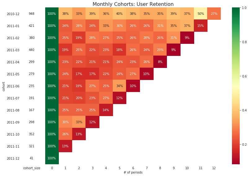
Cohort Analysis:
In this project, we define the cohort group as the customer who purchase on-line within the same months. To translate this idea into cohort analysis, this means we need to group people by their ‘CustomerID’ and ‘InvoiceDate’.
# create two variables: month of order and cohort
data_clean['order_month'] = data_clean['InvoiceDate'].dt.to_period('M')
data_clean['cohort'] = data_clean.groupby('CustomerID')['InvoiceDate'] \
                       .transform('min') \
                       .dt.to_period('M')
data_clean
| InvoiceNo | StockCode | Description | Quantity | InvoiceDate | UnitPrice | CustomerID | Country | date | lowercase_descriptions | Revenue | YearMonth | order_month | cohort | |
|---|---|---|---|---|---|---|---|---|---|---|---|---|---|---|
| 0 | 536365 | 85123A | WHITE HANGING HEART T-LIGHT HOLDER | 6 | 2010-12-01 08:26:00 | 2.55 | 17850.0 | United Kingdom | 2010-12-01 | white hanging heart t-light holder | 15.30 | 201012 | 2010-12 | 2010-12 |
| 1 | 536365 | 71053 | WHITE METAL LANTERN | 6 | 2010-12-01 08:26:00 | 3.39 | 17850.0 | United Kingdom | 2010-12-01 | white metal lantern | 20.34 | 201012 | 2010-12 | 2010-12 |
| 2 | 536365 | 84406B | CREAM CUPID HEARTS COAT HANGER | 8 | 2010-12-01 08:26:00 | 2.75 | 17850.0 | United Kingdom | 2010-12-01 | cream cupid hearts coat hanger | 22.00 | 201012 | 2010-12 | 2010-12 |
| 3 | 536365 | 84029G | KNITTED UNION FLAG HOT WATER BOTTLE | 6 | 2010-12-01 08:26:00 | 3.39 | 17850.0 | United Kingdom | 2010-12-01 | knitted union flag hot water bottle | 20.34 | 201012 | 2010-12 | 2010-12 |
| 4 | 536365 | 84029E | RED WOOLLY HOTTIE WHITE HEART. | 6 | 2010-12-01 08:26:00 | 3.39 | 17850.0 | United Kingdom | 2010-12-01 | red woolly hottie white heart. | 20.34 | 201012 | 2010-12 | 2010-12 |
| ... | ... | ... | ... | ... | ... | ... | ... | ... | ... | ... | ... | ... | ... | ... |
| 541904 | 581587 | 22613 | PACK OF 20 SPACEBOY NAPKINS | 12 | 2011-12-09 12:50:00 | 0.85 | 12680.0 | France | 2011-12-09 | pack of 20 spaceboy napkins | 10.20 | 201112 | 2011-12 | 2011-08 |
| 541905 | 581587 | 22899 | CHILDREN'S APRON DOLLY GIRL | 6 | 2011-12-09 12:50:00 | 2.10 | 12680.0 | France | 2011-12-09 | children's apron dolly girl | 12.60 | 201112 | 2011-12 | 2011-08 |
| 541906 | 581587 | 23254 | CHILDRENS CUTLERY DOLLY GIRL | 4 | 2011-12-09 12:50:00 | 4.15 | 12680.0 | France | 2011-12-09 | childrens cutlery dolly girl | 16.60 | 201112 | 2011-12 | 2011-08 |
| 541907 | 581587 | 23255 | CHILDRENS CUTLERY CIRCUS PARADE | 4 | 2011-12-09 12:50:00 | 4.15 | 12680.0 | France | 2011-12-09 | childrens cutlery circus parade | 16.60 | 201112 | 2011-12 | 2011-08 |
| 541908 | 581587 | 22138 | BAKING SET 9 PIECE RETROSPOT | 3 | 2011-12-09 12:50:00 | 4.95 | 12680.0 | France | 2011-12-09 | baking set 9 piece retrospot | 14.85 | 201112 | 2011-12 | 2011-08 |
406223 rows × 14 columns
# add total number of customers for every time period.
df_cohort = data_clean.groupby(['cohort', 'order_month']) \
              .agg(n_customers=('CustomerID', 'nunique')) \
              .reset_index(drop=False)

# add an indicator for periods (months since first purchase)
df_cohort['period_number'] = (df_cohort.order_month - df_cohort.cohort).\
                              apply(attrgetter('n'))
df_cohort.head(5)
| cohort | order_month | n_customers | period_number | |
|---|---|---|---|---|
| 0 | 2010-12 | 2010-12 | 948 | 0 |
| 1 | 2010-12 | 2011-01 | 362 | 1 |
| 2 | 2010-12 | 2011-02 | 317 | 2 |
| 3 | 2010-12 | 2011-03 | 367 | 3 |
| 4 | 2010-12 | 2011-04 | 341 | 4 |
# pivot the data into a form of the matrix
cohort_pivot = df_cohort.pivot_table(index='cohort',
                                     columns = 'period_number',
                                     values = 'n_customers')
cohort_pivot
| period_number | 0 | 1 | 2 | 3 | 4 | 5 | 6 | 7 | 8 | 9 | 10 | 11 | 12 |
|---|---|---|---|---|---|---|---|---|---|---|---|---|---|
| cohort | |||||||||||||
| 2010-12 | 948.0 | 362.0 | 317.0 | 367.0 | 341.0 | 376.0 | 360.0 | 336.0 | 336.0 | 374.0 | 354.0 | 474.0 | 260.0 |
| 2011-01 | 421.0 | 101.0 | 119.0 | 102.0 | 138.0 | 126.0 | 110.0 | 108.0 | 131.0 | 146.0 | 155.0 | 63.0 | NaN |
| 2011-02 | 380.0 | 94.0 | 73.0 | 106.0 | 102.0 | 94.0 | 97.0 | 107.0 | 98.0 | 119.0 | 34.0 | NaN | NaN |
| 2011-03 | 440.0 | 84.0 | 112.0 | 96.0 | 102.0 | 78.0 | 116.0 | 105.0 | 127.0 | 39.0 | NaN | NaN | NaN |
| 2011-04 | 299.0 | 68.0 | 66.0 | 63.0 | 62.0 | 71.0 | 69.0 | 78.0 | 25.0 | NaN | NaN | NaN | NaN |
| 2011-05 | 279.0 | 66.0 | 48.0 | 48.0 | 60.0 | 68.0 | 74.0 | 29.0 | NaN | NaN | NaN | NaN | NaN |
| 2011-06 | 235.0 | 49.0 | 44.0 | 64.0 | 58.0 | 79.0 | 24.0 | NaN | NaN | NaN | NaN | NaN | NaN |
| 2011-07 | 191.0 | 40.0 | 39.0 | 44.0 | 52.0 | 22.0 | NaN | NaN | NaN | NaN | NaN | NaN | NaN |
| 2011-08 | 167.0 | 42.0 | 42.0 | 42.0 | 23.0 | NaN | NaN | NaN | NaN | NaN | NaN | NaN | NaN |
| 2011-09 | 298.0 | 89.0 | 97.0 | 36.0 | NaN | NaN | NaN | NaN | NaN | NaN | NaN | NaN | NaN |
| 2011-10 | 352.0 | 93.0 | 46.0 | NaN | NaN | NaN | NaN | NaN | NaN | NaN | NaN | NaN | NaN |
| 2011-11 | 321.0 | 43.0 | NaN | NaN | NaN | NaN | NaN | NaN | NaN | NaN | NaN | NaN | NaN |
| 2011-12 | 41.0 | NaN | NaN | NaN | NaN | NaN | NaN | NaN | NaN | NaN | NaN | NaN | NaN |
# divide by the cohort size (month 0) to obtain retention as %
cohort_size = cohort_pivot.iloc[:,0]
retention_matrix = cohort_pivot.divide(cohort_size, axis = 0)
# plot the rentention matrix
with sns.axes_style("white"):
    fig, ax = plt.subplots(1, 2, figsize=(12, 8), sharey=True, \
                           gridspec_kw={'width_ratios': [1, 11]})

    # retention matrix
    sns.heatmap(retention_matrix,
                mask=retention_matrix.isnull(),
                annot=True,
                fmt='.0%',
                cmap='RdYlGn',
                ax=ax[1])
    ax[1].set_title('Monthly Cohorts: User Retention', fontsize=16)
    ax[1].set(xlabel='# of periods',
              ylabel='')


    # cohort size
    cohort_size_df = pd.DataFrame(cohort_size).rename(columns={0: 'cohort_size'})
    white_cmap = mcolors.ListedColormap(['white'])
    sns.heatmap(cohort_size_df,
                annot=True,
                cbar=False,
                fmt='g',
                cmap=white_cmap,
                ax=ax[0])

    fig.tight_layout()